Unpivot Excel data with Python

This post is is based on another demo from my SQLSaturday session on Python integration in Power BI. Its a handy real world scenario that could easily be re-applied with minor changes to the script. The primary pattern is unpivot functionality which is achieved through the melt method in pandas.  A few additional useful dataframe techniques are illustrated, including pivot_table.

I am using the Tourist Accommodation data from the Statistics South Africa website. The file (tourism.xlsx) is also available on the SQLSaturday website. Once you open the file observe the following:

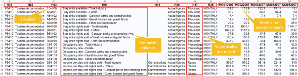
• the first 8 columns (starting with the letter H) are the header columns
• the remaining columns are a series of months i.e. MO012007 is month 1 (Jan), 2007
• the numeric values have mixed scale including thousands, millions & percentages
• column H04 is a mix of metric and accommodation type

The Python script will provide a way to transform the data even if the columns increase as months get added.

Step 1: Load Excel data into a dataframe

import pandas
df = pandas.read_excel('D:\\data\\excel\\tourism.xlsx')

The read_excel method accepts a host of parameters, including specifying the sheet_name. Our Excel file has only 1 sheet, so the sheet_name is not required.

Step 2: Split columns into actual headers and months

We start by adding the dataframe columns to a list. Then we loop through the list and split the month columns from the actual headers.

#create a list of all the columns
columns = list(df)
#create lists to hold headers & months
headers = []
months = []
#split columns list into headers and months
for col in columns:
    if col.startswith('MO'):
        months.append(col)
    else:
        headers.append(col)

Here we have the best case scenario because all month columns start with “MO”. If no pattern exists and the columns are sequenced, you could split on position i.e. headers = columns[:8], months = columns[8:] will produce the same result. Worst scenario is when the order of the columns are random. In this case you would manually specify the list elements.

Step 3: Melt (unpivot) the month columns

Unpivoting will transpose all month columns to rows. For each month column a new row is created using the same header columns.

df2 = pandas.melt(df,
                  id_vars=headers,
                  value_vars=months,
                  var_name='Date',
                  value_name='Val')

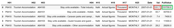
All month columns will be dropped and a new column ‘Date’ will contain the original month column header. The values will bed added to a new column called ‘Val’.

Now reconstruct and convert the Date column to an actual date. We get the year and month parts from the column and just assume the day is always 1. This is explicitly converted to a date using the to_datetime method.

df2['Date'] = pandas.to_datetime(df2['Date'].str[4:9] + '-' + df2['Date'].str[2:4] + '-01')

Step 4: Standardize the values 

We noted at the start that the values were a mixture of numeric scales which is indicated in column H17. To determine the possible value scales we use df2.H17.unique() which returns the following list of unique values: [‘Thousand’, ‘Percentage’, ‘Rands’, ‘R million’]. We create a function to apply the scale to the Val column.

 def noscale(row):
    if row['H17'] == 'Thousand':
        return row['Val'] * 1000
    elif row['H17'] =='R million':
        return row['Val'] * 1000000
    elif row['H17'] =='Percentage':
        return row['Val'] / 100
    else:
        return row['Val']

df2['FullValue'] = df2.apply(noscale, axis=1)

“Rands” are just the local currency (ZAR), so no scale is required.

Step 5: Additional clean up 

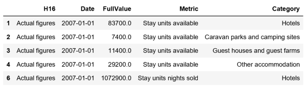
The next 3 steps in our script splits the composite column and removes unwanted rows and columns.

#split composite column
df2['Metric'] = df2['H04'].str.split(' - ').str.get(0)
df2['Category'] = df2['H04'].str.split(' - ').str.get(1)
#remove aggregate rows
df2 = df2[df2.Category != 'Total industry']
#remove unwanted columns
df2 = df2.drop(['H01','H02','H03','H04','H15','H17','H25','Val'], axis=1)

Note how rows are filtered. We set the dataframe equal to the existing dataframe where the Category column is not equal to ‘Total Industry’

At this point the script could be used as is, but in Power BI we would need to understand how the measure(s) would be created. For example, we could have a generic measure [Value] = SUM(‘Tourism'[FullValue]). We would then use the Metric column as a filter/slicer. Most likely you would rather want a measure such as [Units Available] = CALCULATE ( SUM ( ‘Tourism'[FullValue] ), ‘Tourism'[Metric]=”Stay units available” ). In this case it is cumbersome to create the measures, so we rather reshape the table to make things easier.

Step 6: Pivot the Metrics (optional)

If the metrics provided are fixed (consistent), then pivoting the metrics  is a good idea. This creates a column for each metric. This is possible with the Pandas pivot_table method.

df3 = pandas.pivot_table(df2,
                         values='FullValue',
                         columns=['Metric'],
                         index=['H16','Date','Category'])

From the results below, this appears to be correct.

The side effect of the pivot_table method is that the dataframe is re-indexed based on the index parameter passed to the method. This is not really a problem, but for Power BI it is. You may have noted from earlier posts that the Python Script in Power BI does not provide access to the dataframe index. So we would in effect lose the first three columns from our result above.

The fix is as simple as re-indexing the dataframe. We can also drop the ‘Total income’ column as we can let Power BI handle the aggregations.

df3.reset_index(inplace=True)
df3 = df3.drop(['Total income'], axis=1)

Our final script below will produce 3 dataframes which will be available for selection in Power BI.

import pandas

#read Excel into dataframe
df = pandas.read_excel('D:\\data\\excel\\tourism.xlsx')

#create place holder lists for actaul headers vs months
headers = []
months = []

#split columns into headers and months
for col in list(df):
    if col.startswith('MO'):
        months.append(col)
    else:
        headers.append(col)

#unpivot months
df2 = pandas.melt(df,
                  id_vars=headers,
                  value_vars=months,
                  var_name='Date',
                  value_name='Val')

#create a date field from the month field
df2['Date'] = pandas.to_datetime(df2['Date'].str[4:] + '-' + df2['Date'].str[2:4] + '-01')

#create a function to resolve mixed numeric scale in the data
def noscale(row):
    if row['H17'] == 'Thousand':
        return row['Val'] * 1000
    elif row['H17'] =='R million':
        return row['Val'] * 1000000
    elif row['H17'] =='Percentage':
        return row['Val'] / 100
    else:
        return row['Val']

#apply the noscale function to the dataframe
df2['FullValue'] = df2.apply(noscale, axis=1)

#split composite column
df2['Metric'] = df2['H04'].str.split(' - ').str.get(0)
df2['Category'] = df2['H04'].str.split(' - ').str.get(1)
#remove aggregate rows
df2 = df2[df2.Category != 'Total industry']
#remove unwanted columns
df2 = df2.drop(['H01','H02','H03','H04','H15','H17','H25','Val'], axis=1)

#unpivot metrics
df3 = pandas.pivot_table(df2,
                         values='FullValue',
                         columns=['Metric'],
                         index=['H16','Date','Category'])
#reset index
df3.reset_index(inplace=True)
#drop aggregate column
df3 = df3.drop(['Total income'], axis=1)

All that is left is to paste your script into Power BI and select the dataframe that works best for you.

Of course go and experiment with Python visualization 😊